SenLand
SenLand — Senegal's land cover with deep learning
A real AI project, actually run — entirely on a single laptop, with the techniques taught at the Gray Scott School (CINERI). The same neural network maps land cover — water, cropland, forest, built-up, mangroves — from open satellite imagery. The engineering question that shapes the whole project: run this code first on the CPU, then on the GPU of the same machine, and compare the two compute engines honestly — their architecture, how you exploit them, their limits, and the measured results.
The problem
Knowing where cropland, water, forests and cities are — and how they change year to year — is a national question: agriculture, water resources, urbanization, climate. Manual mapping does not scale to a country. A neural network learns to read satellite imagery and produces the map automatically, everywhere, at the same resolution.
The pipeline, end to end
Four stages: read the open data (imagery + labels), tile it into small patches, a U-Net segments each patch, and the land-cover map is recomposed.
The data (100% open)
Sentinel-2 imagery (cloudless, 10 m) pixel-aligned with ESA WorldCover labels (10 m). Four deliberately different landscapes, read live from public servers — no private data, no bulk download.
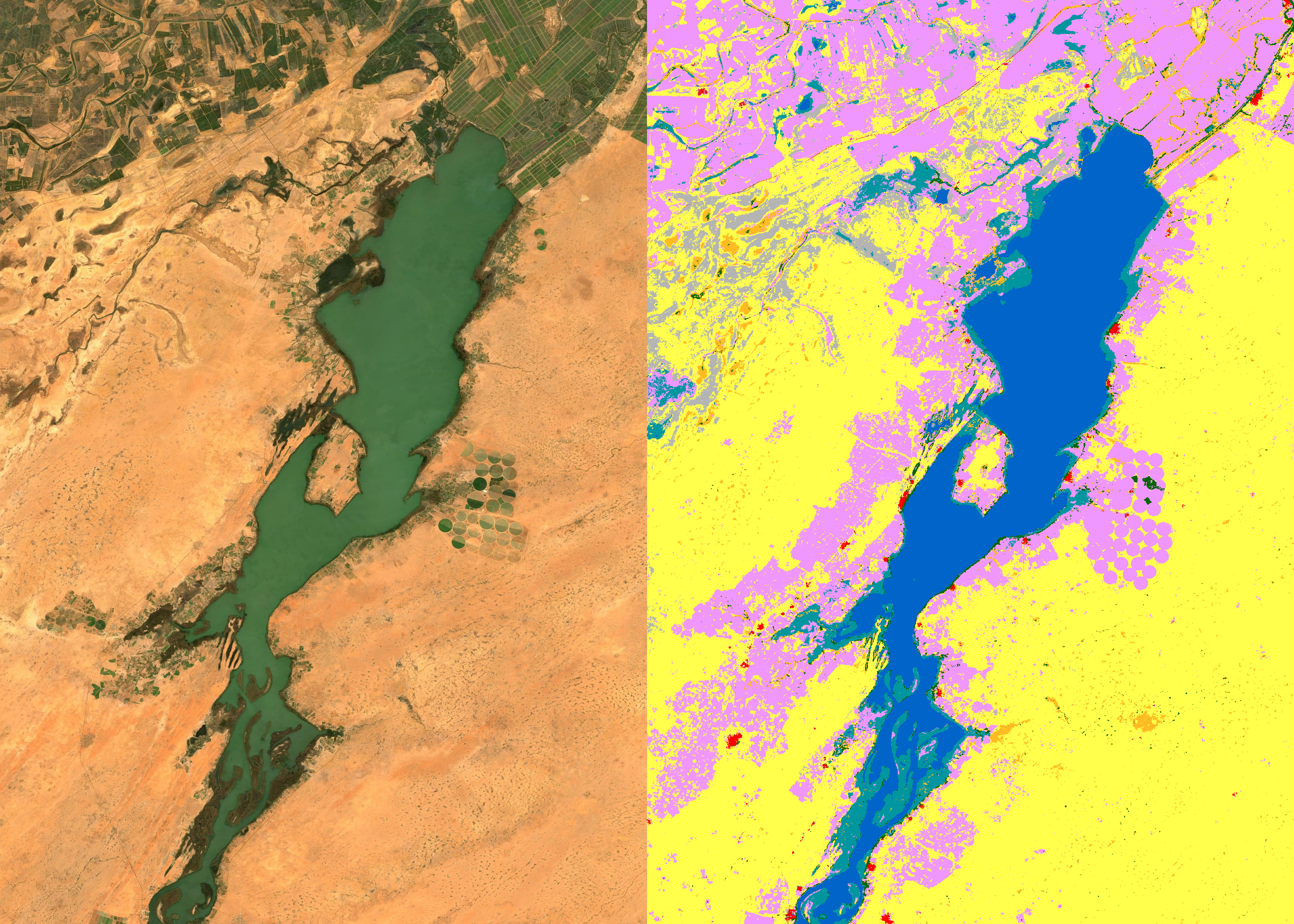
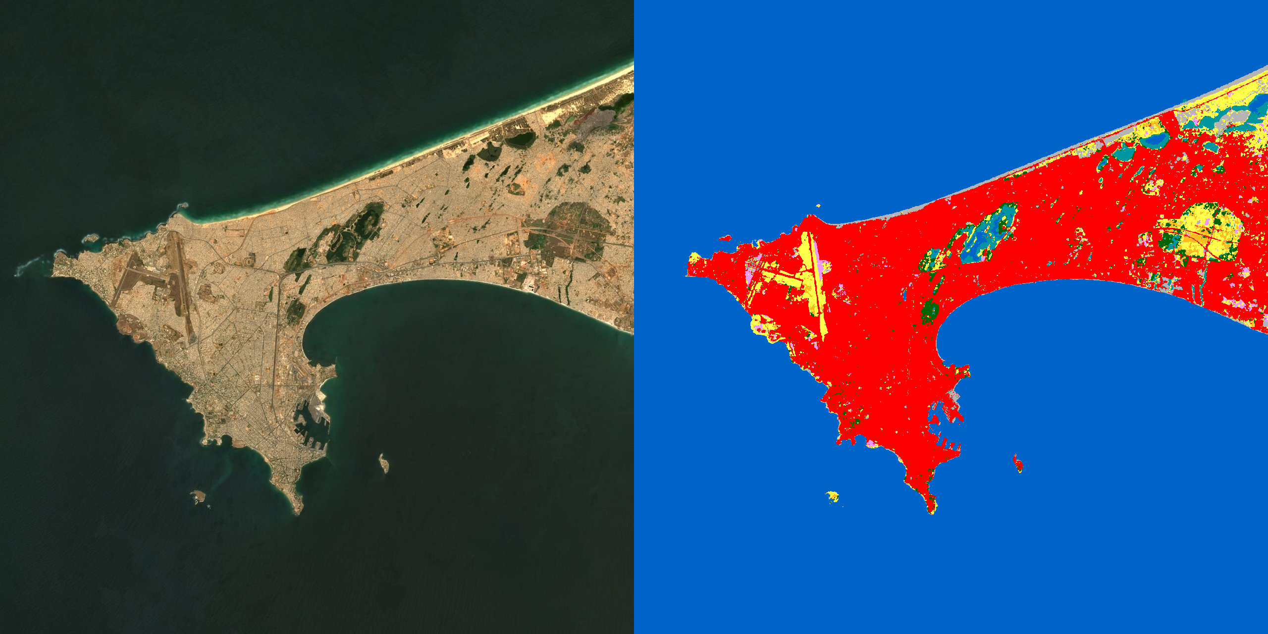
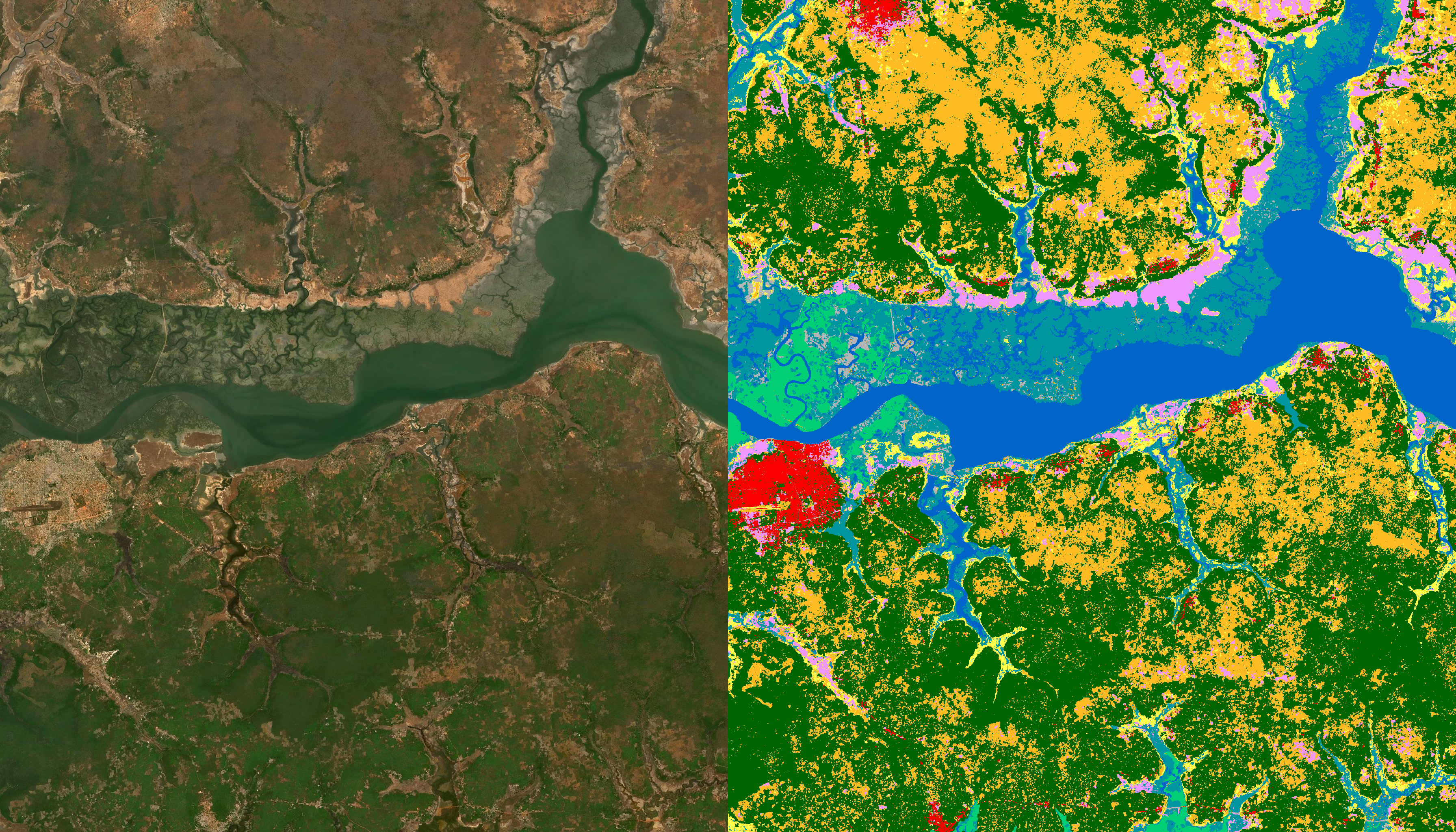
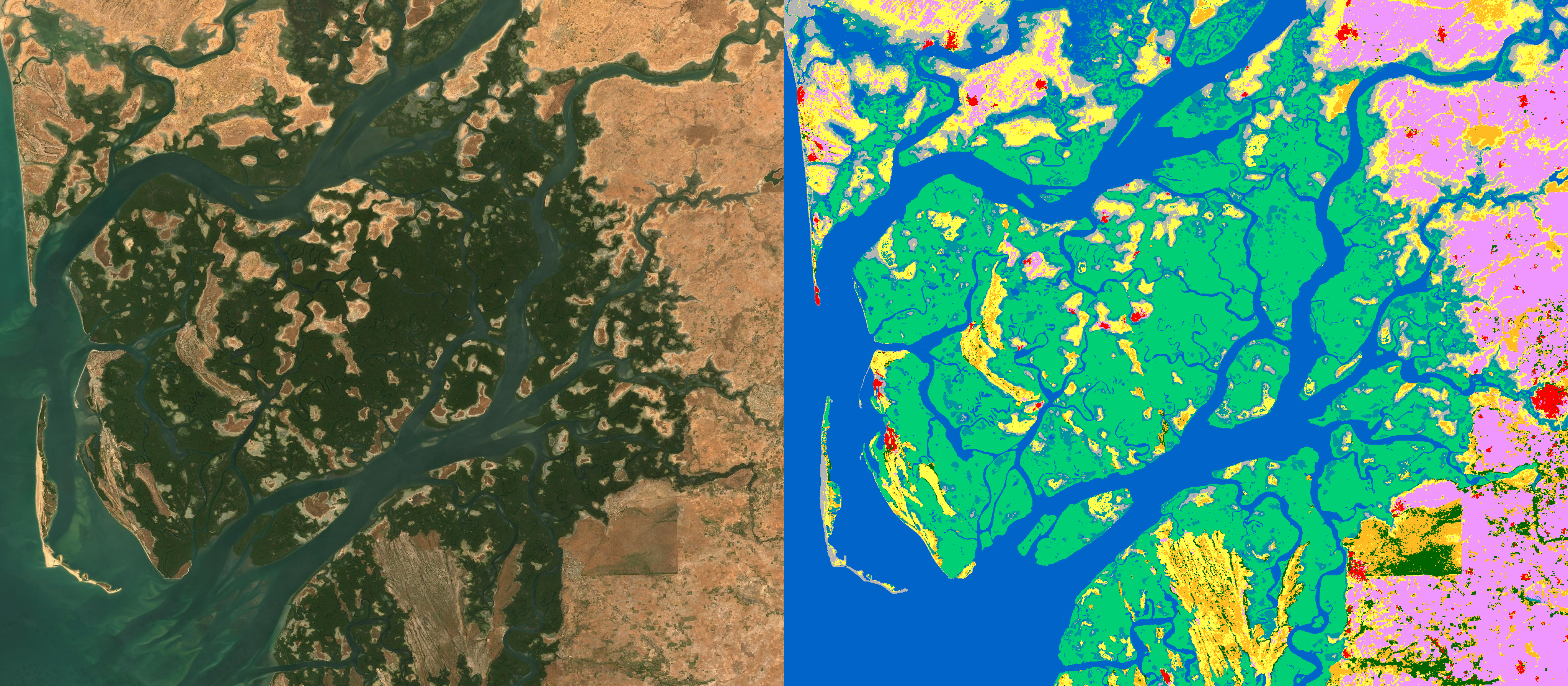
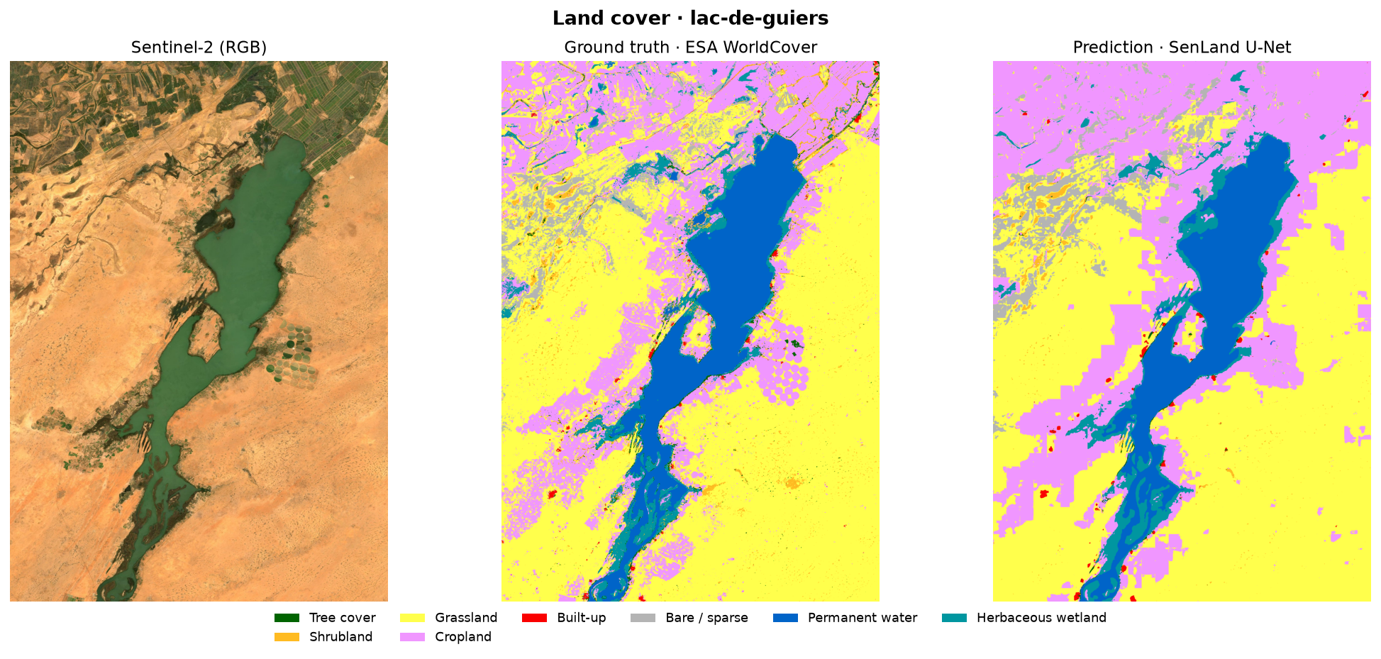
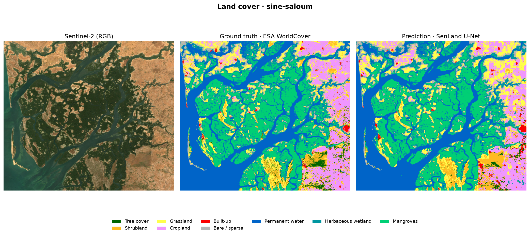
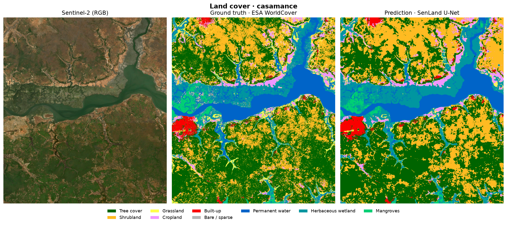
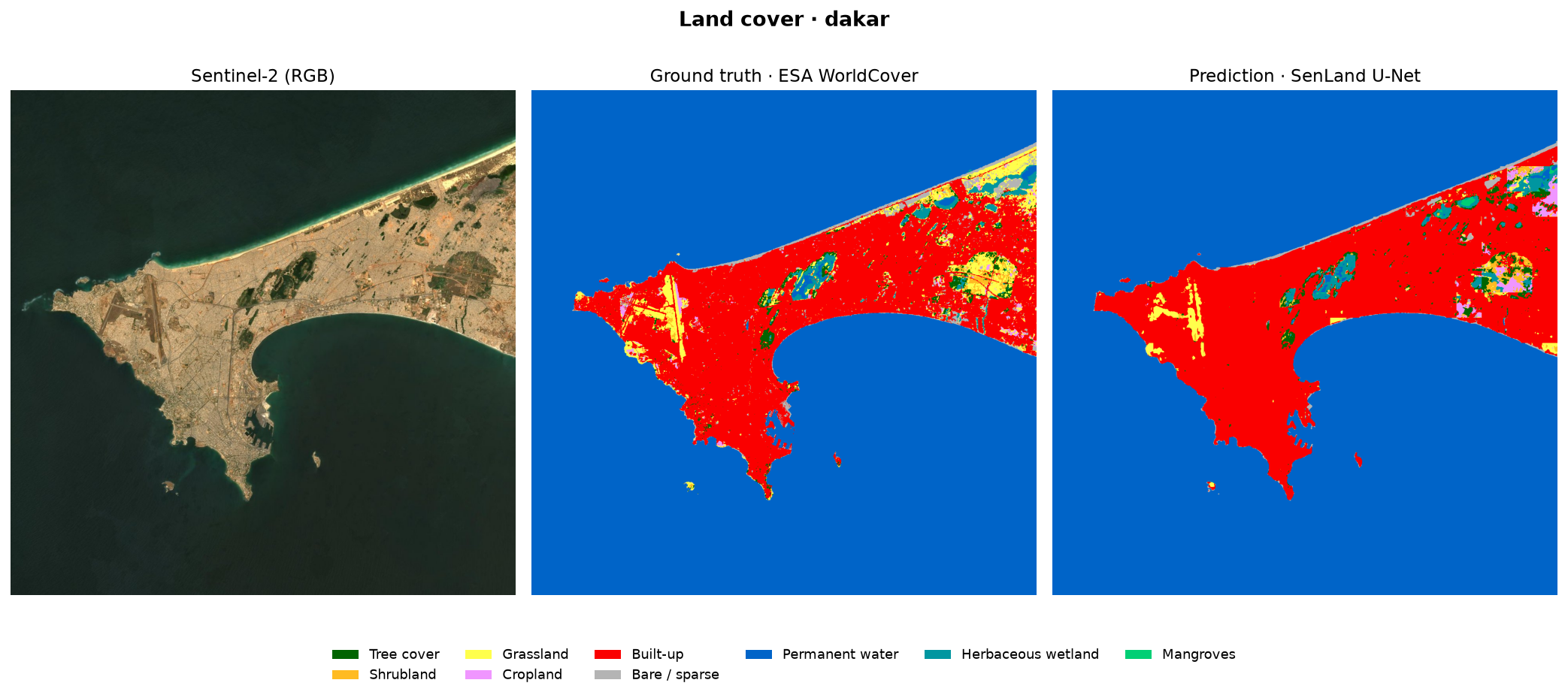
Results — the maps
For each area: the Sentinel-2 image, the ground truth (WorldCover) and the model's prediction, side by side. The lake, the ocean and the large agricultural structures are faithfully reconstructed.
Metrics
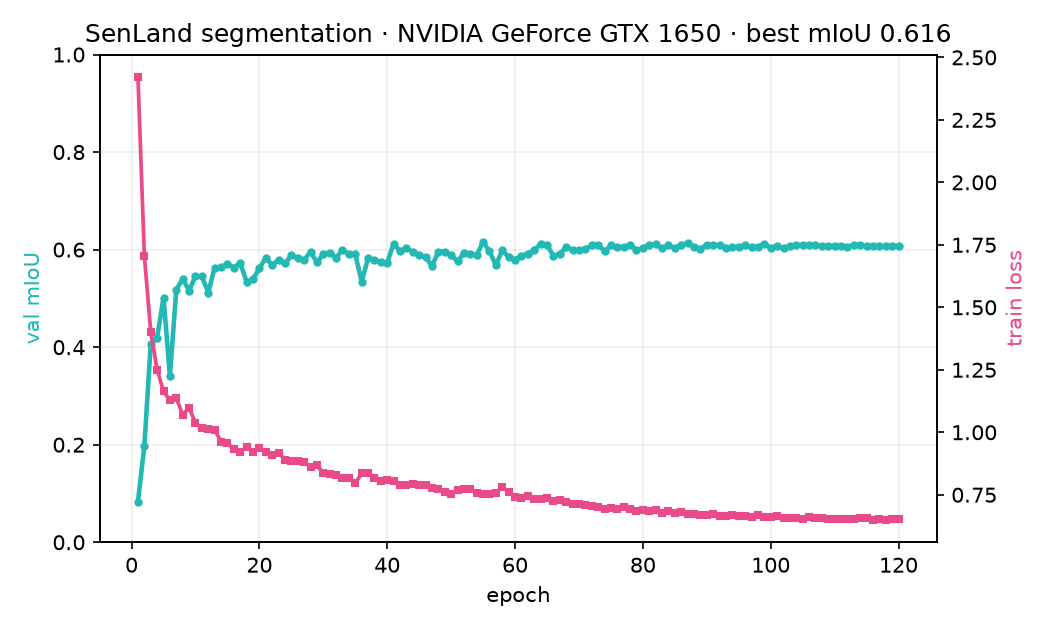
Segmentation is evaluated on a spatial holdout (a validation area kept apart, for an honest measure of generalization).
| Task | Metric | Value |
|---|---|---|
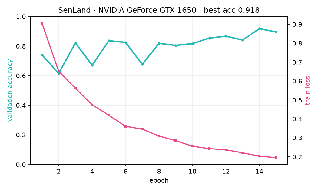
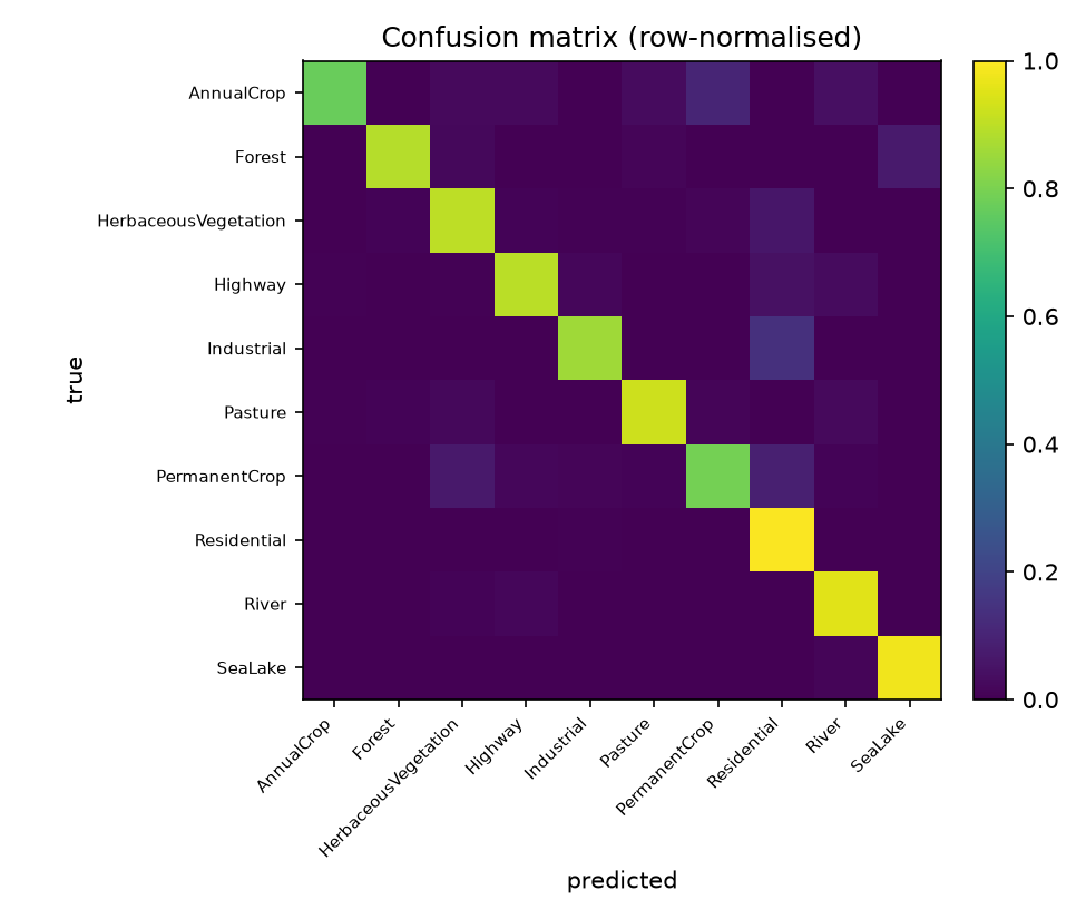
| Classification (EuroSAT, 10 classes, from scratch) | validation accuracy | 91.8% |
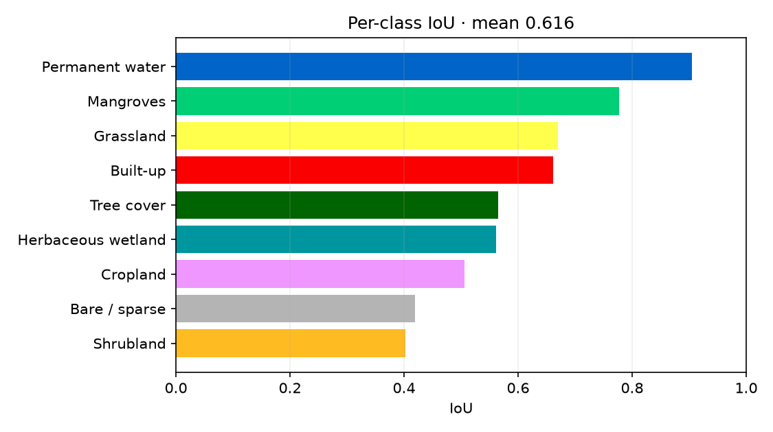
| Segmentation (4 areas, spatial holdout) | mean IoU | 0.62 |
Adding the Saloum delta to training lifts mangroves from 3% to 83% IoU — the demonstration that the right data beats a bigger model.
The architecture — one code, two engines
The model is a U-Net (ResNet-34 encoder) for segmentation, preceded by a ResNet-18 for the
classification warm-up, all in PyTorch. The core of the project reuses the Kokkos idea
from Day 4: one source, two backends. It is exactly the same code that runs on the CPU or the
GPU — a hardware introspection layer (hw.py) picks the device and declares it honestly in
every figure, never a CPU run labeled "GPU".
On CPU, parallelism goes through OpenMP intra-op threads (Day 1 / TBB); on GPU, through the massive SIMT parallelism of CUDA cores (Day 2 / 3). No line of science changes: only the iteration throughput does.
On CPU
No GPU required: the same code uses all cores via OpenMP threads. Strong scaling measured on the laptop (Intel i5-10300H, 1 → 8 threads). Efficiency drops beyond 4 threads: the machine has only 4 physical cores, HyperThreading doesn't help dense compute.
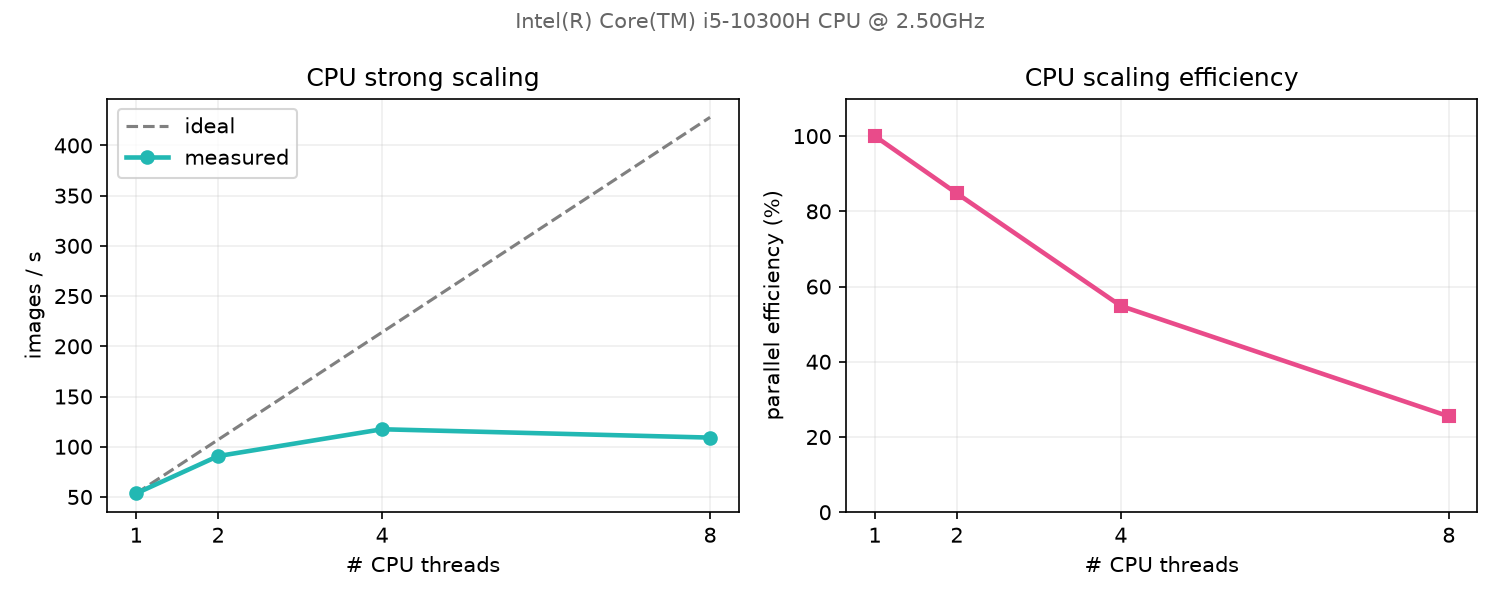
- Pros — available everywhere (no specialized hardware); plenty of RAM, ideal for geo I/O
(
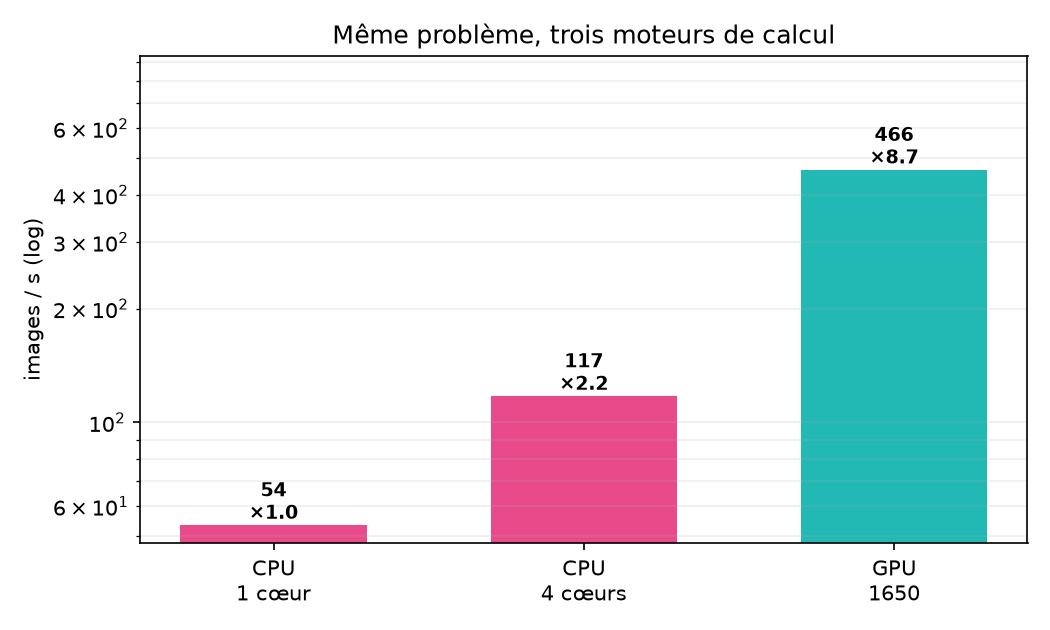
/vsicurlreads of Sentinel-2 + WorldCover); simple, reproducible debugging; real strong scaling (×2.2 from 1 to 4 cores, 54 → 117 img/s). - Cons — caps at 4 physical cores (HyperThreading adds nothing: 117 → 109 img/s); ≈ 4× slower than the same machine's modest GPU; an epoch in ~25 s vs ~5 s on GPU.
Same weights, same model quality — only slower. The CPU produces exactly the same science, at a lower throughput.
On GPU
The GPU applies massive parallelism (SIMT): thousands of CUDA cores process the batch at once. On the laptop's GTX 1650, throughput reaches 466 img/s, iteration becomes fluid — which enabled the long training runs (120 segmentation epochs).
- Pros — ≈ ×4 faster than the best CPU, ×8.6 vs a single core; fluid iteration (5.5 s/epoch); architecture built for dense convolutions — SIMT fits the model.
- Cons — limited VRAM (4 GB), constraining batch and tile size; mixed precision (AMP fp16) diverges to NaN on this consumer card — disabled locally (an honest limit); host→device transfer overhead.
Strictly the same model and final accuracy as on CPU — the GPU doesn't change the result, it delivers it ~4× faster. The gain is entirely engineer time recovered.
Head to head — measured throughput
Same problem, same code, three engines of the same machine. Everything is measured here, on the laptop — nothing is projected.
The JAX port — comparing frameworks, not just engines
A direct extension of the school's Days 5 and 7 (Python on CPU, then on GPU): the same
segmentation task is reimplemented in JAX/Flax (src/senland_jax/) to compare frameworks
on top of engines — same Senegal areas, same IoU yardstick. The model is a from-scratch
U-Net (GroupNorm, 7.8 M parameters, no ImageNet pretraining); the training step is a pure
function compiled with jax.jit and differentiated with jax.value_and_grad.
| Framework | Engine | mIoU | Throughput |
|---|---|---|---|
| PyTorch — U-Net ResNet-34, ImageNet | GPU GTX 1650 | 0.62 | 470 patch/s |
| JAX — U-Net GroupNorm, from scratch | GPU GTX 1650 | 0.57 | 211 patch/s |
| JAX — same model | CPU i5-10300H | — | 13 patch/s |
Reading these numbers honestly:
- mIoU 0.57 vs 0.62 — the gap is the ImageNet-pretrained encoder on the PyTorch side; the JAX model trains from scratch. Per-class IoU still tracks closely (permanent water 0.90 vs 0.91, mangroves 0.77 vs 0.78).
- The "one code, two engines" story holds in JAX too: the same jitted code runs
≈ ×16 faster on GPU than on CPU — here via device placement (
JAX_PLATFORMS) rather thanhw.py.
Same JAX code, device placement via JAX_PLATFORMS — ≈ ×16 on GPU.
The fair benchmark — identical model in both frameworks
Comparing a pretrained ResNet-34 to a small hand-written U-Net is not a fair race.
scripts/bench_unet.py therefore builds the strictly identical U-Net (GroupNorm, 11
classes) in both frameworks and times the full training step (forward + CE+Dice + backward
- AdamW) on a device-resident batch — isolating the framework/compiler from the architecture. GTX 1650, fp32:
| Mode | batch 8 | batch 16 |
|---|---|---|
JAX — naive (per-step jit) | 246 | — |
| PyTorch — eager | 334 | — |
PyTorch — torch.compile | 356 | 460 |
JAX — fused multi-step (lax.fori_loop) | 371 | 463 |
(patches/s; higher is better)
Identical GroupNorm U-Net in both frameworks, full training step, GTX 1650 fp32.
Takeaways:
- Naive JAX (one dispatch per step) is the slowest. Once its real levers are engaged —
jit,donate_argnums(buffer reuse), device-resident inputs, and above all step fusion (lax.fori_loop: 20 steps for the cost of one dispatch) — JAX edges pasttorch.compileat batch 8 (+4%) and ties it at batch 16. - At an identical model, fully-tuned JAX ≈ fully-tuned PyTorch on this card. The earlier ~2× gap was the architecture (smp ResNet-34 vs a hand-written U-Net), not the framework. XLA's advantage would widen on TPUs, larger batches/models, or more fusable graphs — none of which a 4 GB consumer GPU exercises.
Honest reproduction pitfall:
jax[cuda12]and PyTorch pin differentnvidia-cudnn-cu12versions — in one shared venv only one of the two has working GPU at a time. Use two separate environments.
Built with the Gray Scott School techniques
Every engineering brick of SenLand reuses a technique from the Gray Scott School (CINERI) and applies it to deep learning. The through-line — one code, CPU then GPU — is the very idea of Kokkos.
| Brick | School day |
|---|---|
| One code, two backends | Day 4 · Kokkos → here hw.py (PyTorch) and JAX_PLATFORMS (JAX) |
| Frameworks & compilers | Days 5 & 7 · Python/JAX — jit, XLA, step fusion (fori_loop) |
| Multicore CPU | Day 1 · parallelism + Day 2 · TBB — shared memory, strong scaling |
| GPU SIMT / CUDA | Day 2 · GPU + Day 3 · CUDA — massive parallelism |
| Benchmark & timing | Day 2 · fixed workload, img/s throughput |
| Vectorization / SIMD | Day 1 + Day 6 · EVE — mixed-precision (AMP) analogue |
| Floating-point precision | Day 3 · fp32/fp16 — explains the AMP NaN on GTX 1650 |
| I/O & data | Day 2 · HDF5 → here geo I/O Sentinel-2 / WorldCover |
| Containers & repro | pixi / Apptainer — fixed seeds, versioned experiments |
SenLand is an open, reproducible project: every number on this page is backed by a figure committed to the repository. The code runs without a GPU; with one, everything simply goes ~4× faster.